1211 lines
28 KiB
Markdown
1211 lines
28 KiB
Markdown
|
||
# Datawhale 零基础入门数据挖掘-Baseline
|
||
|
||
## Baseline-v1.0 版
|
||
|
||
Tip:这是一个最初始baseline版本,抛砖引玉,为大家提供一个基本Baseline和一个竞赛流程的基本介绍,欢迎大家多多交流。
|
||
|
||
**赛题:零基础入门数据挖掘 - 二手车交易价格预测**
|
||
|
||
地址:https://tianchi.aliyun.com/competition/entrance/231784/introduction?spm=5176.12281957.1004.1.38b02448ausjSX
|
||
|
||
|
||
```python
|
||
# 查看数据文件目录 list datalab files
|
||
!ls datalab/
|
||
```
|
||
|
||
231784
|
||
|
||
|
||
### Step 1:导入函数工具箱
|
||
|
||
|
||
```python
|
||
## 基础工具
|
||
import numpy as np
|
||
import pandas as pd
|
||
import warnings
|
||
import matplotlib
|
||
import matplotlib.pyplot as plt
|
||
import seaborn as sns
|
||
from scipy.special import jn
|
||
from IPython.display import display, clear_output
|
||
import time
|
||
|
||
warnings.filterwarnings('ignore')
|
||
%matplotlib inline
|
||
|
||
## 模型预测的
|
||
from sklearn import linear_model
|
||
from sklearn import preprocessing
|
||
from sklearn.svm import SVR
|
||
from sklearn.ensemble import RandomForestRegressor,GradientBoostingRegressor
|
||
|
||
## 数据降维处理的
|
||
from sklearn.decomposition import PCA,FastICA,FactorAnalysis,SparsePCA
|
||
|
||
import lightgbm as lgb
|
||
import xgboost as xgb
|
||
|
||
## 参数搜索和评价的
|
||
from sklearn.model_selection import GridSearchCV,cross_val_score,StratifiedKFold,train_test_split
|
||
from sklearn.metrics import mean_squared_error, mean_absolute_error
|
||
```
|
||
|
||
### Step 2:数据读取
|
||
|
||
|
||
```python
|
||
## 通过Pandas对于数据进行读取 (pandas是一个很友好的数据读取函数库)
|
||
Train_data = pd.read_csv('datalab/231784/used_car_train_20200313.csv', sep=' ')
|
||
TestA_data = pd.read_csv('datalab/231784/used_car_testA_20200313.csv', sep=' ')
|
||
|
||
## 输出数据的大小信息
|
||
print('Train data shape:',Train_data.shape)
|
||
print('TestA data shape:',TestA_data.shape)
|
||
```
|
||
|
||
Train data shape: (150000, 31)
|
||
TestA data shape: (50000, 30)
|
||
|
||
|
||
#### 1) 数据简要浏览
|
||
|
||
|
||
```python
|
||
## 通过.head() 简要浏览读取数据的形式
|
||
Train_data.head()
|
||
```
|
||
|
||
|
||
|
||
|
||
<div>
|
||
<style scoped>
|
||
.dataframe tbody tr th:only-of-type {
|
||
vertical-align: middle;
|
||
}
|
||
|
||
.dataframe tbody tr th {
|
||
vertical-align: top;
|
||
}
|
||
|
||
.dataframe thead th {
|
||
text-align: right;
|
||
}
|
||
</style>
|
||
<table border="1" class="dataframe">
|
||
<thead>
|
||
<tr style="text-align: right;">
|
||
<th></th>
|
||
<th>SaleID</th>
|
||
<th>name</th>
|
||
<th>regDate</th>
|
||
<th>model</th>
|
||
<th>brand</th>
|
||
<th>bodyType</th>
|
||
<th>fuelType</th>
|
||
<th>gearbox</th>
|
||
<th>power</th>
|
||
<th>kilometer</th>
|
||
<th>...</th>
|
||
<th>v_5</th>
|
||
<th>v_6</th>
|
||
<th>v_7</th>
|
||
<th>v_8</th>
|
||
<th>v_9</th>
|
||
<th>v_10</th>
|
||
<th>v_11</th>
|
||
<th>v_12</th>
|
||
<th>v_13</th>
|
||
<th>v_14</th>
|
||
</tr>
|
||
</thead>
|
||
<tbody>
|
||
<tr>
|
||
<th>0</th>
|
||
<td>0</td>
|
||
<td>736</td>
|
||
<td>20040402</td>
|
||
<td>30.0</td>
|
||
<td>6</td>
|
||
<td>1.0</td>
|
||
<td>0.0</td>
|
||
<td>0.0</td>
|
||
<td>60</td>
|
||
<td>12.5</td>
|
||
<td>...</td>
|
||
<td>0.235676</td>
|
||
<td>0.101988</td>
|
||
<td>0.129549</td>
|
||
<td>0.022816</td>
|
||
<td>0.097462</td>
|
||
<td>-2.881803</td>
|
||
<td>2.804097</td>
|
||
<td>-2.420821</td>
|
||
<td>0.795292</td>
|
||
<td>0.914762</td>
|
||
</tr>
|
||
<tr>
|
||
<th>1</th>
|
||
<td>1</td>
|
||
<td>2262</td>
|
||
<td>20030301</td>
|
||
<td>40.0</td>
|
||
<td>1</td>
|
||
<td>2.0</td>
|
||
<td>0.0</td>
|
||
<td>0.0</td>
|
||
<td>0</td>
|
||
<td>15.0</td>
|
||
<td>...</td>
|
||
<td>0.264777</td>
|
||
<td>0.121004</td>
|
||
<td>0.135731</td>
|
||
<td>0.026597</td>
|
||
<td>0.020582</td>
|
||
<td>-4.900482</td>
|
||
<td>2.096338</td>
|
||
<td>-1.030483</td>
|
||
<td>-1.722674</td>
|
||
<td>0.245522</td>
|
||
</tr>
|
||
<tr>
|
||
<th>2</th>
|
||
<td>2</td>
|
||
<td>14874</td>
|
||
<td>20040403</td>
|
||
<td>115.0</td>
|
||
<td>15</td>
|
||
<td>1.0</td>
|
||
<td>0.0</td>
|
||
<td>0.0</td>
|
||
<td>163</td>
|
||
<td>12.5</td>
|
||
<td>...</td>
|
||
<td>0.251410</td>
|
||
<td>0.114912</td>
|
||
<td>0.165147</td>
|
||
<td>0.062173</td>
|
||
<td>0.027075</td>
|
||
<td>-4.846749</td>
|
||
<td>1.803559</td>
|
||
<td>1.565330</td>
|
||
<td>-0.832687</td>
|
||
<td>-0.229963</td>
|
||
</tr>
|
||
<tr>
|
||
<th>3</th>
|
||
<td>3</td>
|
||
<td>71865</td>
|
||
<td>19960908</td>
|
||
<td>109.0</td>
|
||
<td>10</td>
|
||
<td>0.0</td>
|
||
<td>0.0</td>
|
||
<td>1.0</td>
|
||
<td>193</td>
|
||
<td>15.0</td>
|
||
<td>...</td>
|
||
<td>0.274293</td>
|
||
<td>0.110300</td>
|
||
<td>0.121964</td>
|
||
<td>0.033395</td>
|
||
<td>0.000000</td>
|
||
<td>-4.509599</td>
|
||
<td>1.285940</td>
|
||
<td>-0.501868</td>
|
||
<td>-2.438353</td>
|
||
<td>-0.478699</td>
|
||
</tr>
|
||
<tr>
|
||
<th>4</th>
|
||
<td>4</td>
|
||
<td>111080</td>
|
||
<td>20120103</td>
|
||
<td>110.0</td>
|
||
<td>5</td>
|
||
<td>1.0</td>
|
||
<td>0.0</td>
|
||
<td>0.0</td>
|
||
<td>68</td>
|
||
<td>5.0</td>
|
||
<td>...</td>
|
||
<td>0.228036</td>
|
||
<td>0.073205</td>
|
||
<td>0.091880</td>
|
||
<td>0.078819</td>
|
||
<td>0.121534</td>
|
||
<td>-1.896240</td>
|
||
<td>0.910783</td>
|
||
<td>0.931110</td>
|
||
<td>2.834518</td>
|
||
<td>1.923482</td>
|
||
</tr>
|
||
</tbody>
|
||
</table>
|
||
<p>5 rows × 31 columns</p>
|
||
</div>
|
||
|
||
|
||
|
||
#### 2) 数据信息查看
|
||
|
||
|
||
```python
|
||
## 通过 .info() 简要可以看到对应一些数据列名,以及NAN缺失信息
|
||
Train_data.info()
|
||
```
|
||
|
||
<class 'pandas.core.frame.DataFrame'>
|
||
RangeIndex: 150000 entries, 0 to 149999
|
||
Data columns (total 31 columns):
|
||
SaleID 150000 non-null int64
|
||
name 150000 non-null int64
|
||
regDate 150000 non-null int64
|
||
model 149999 non-null float64
|
||
brand 150000 non-null int64
|
||
bodyType 145494 non-null float64
|
||
fuelType 141320 non-null float64
|
||
gearbox 144019 non-null float64
|
||
power 150000 non-null int64
|
||
kilometer 150000 non-null float64
|
||
notRepairedDamage 150000 non-null object
|
||
regionCode 150000 non-null int64
|
||
seller 150000 non-null int64
|
||
offerType 150000 non-null int64
|
||
creatDate 150000 non-null int64
|
||
price 150000 non-null int64
|
||
v_0 150000 non-null float64
|
||
v_1 150000 non-null float64
|
||
v_2 150000 non-null float64
|
||
v_3 150000 non-null float64
|
||
v_4 150000 non-null float64
|
||
v_5 150000 non-null float64
|
||
v_6 150000 non-null float64
|
||
v_7 150000 non-null float64
|
||
v_8 150000 non-null float64
|
||
v_9 150000 non-null float64
|
||
v_10 150000 non-null float64
|
||
v_11 150000 non-null float64
|
||
v_12 150000 non-null float64
|
||
v_13 150000 non-null float64
|
||
v_14 150000 non-null float64
|
||
dtypes: float64(20), int64(10), object(1)
|
||
memory usage: 35.5+ MB
|
||
|
||
|
||
|
||
```python
|
||
## 通过 .columns 查看列名
|
||
Train_data.columns
|
||
```
|
||
|
||
|
||
|
||
|
||
Index(['SaleID', 'name', 'regDate', 'model', 'brand', 'bodyType', 'fuelType',
|
||
'gearbox', 'power', 'kilometer', 'notRepairedDamage', 'regionCode',
|
||
'seller', 'offerType', 'creatDate', 'price', 'v_0', 'v_1', 'v_2', 'v_3',
|
||
'v_4', 'v_5', 'v_6', 'v_7', 'v_8', 'v_9', 'v_10', 'v_11', 'v_12',
|
||
'v_13', 'v_14'],
|
||
dtype='object')
|
||
|
||
|
||
|
||
|
||
```python
|
||
TestA_data.info()
|
||
```
|
||
|
||
<class 'pandas.core.frame.DataFrame'>
|
||
RangeIndex: 50000 entries, 0 to 49999
|
||
Data columns (total 30 columns):
|
||
SaleID 50000 non-null int64
|
||
name 50000 non-null int64
|
||
regDate 50000 non-null int64
|
||
model 50000 non-null float64
|
||
brand 50000 non-null int64
|
||
bodyType 48587 non-null float64
|
||
fuelType 47107 non-null float64
|
||
gearbox 48090 non-null float64
|
||
power 50000 non-null int64
|
||
kilometer 50000 non-null float64
|
||
notRepairedDamage 50000 non-null object
|
||
regionCode 50000 non-null int64
|
||
seller 50000 non-null int64
|
||
offerType 50000 non-null int64
|
||
creatDate 50000 non-null int64
|
||
v_0 50000 non-null float64
|
||
v_1 50000 non-null float64
|
||
v_2 50000 non-null float64
|
||
v_3 50000 non-null float64
|
||
v_4 50000 non-null float64
|
||
v_5 50000 non-null float64
|
||
v_6 50000 non-null float64
|
||
v_7 50000 non-null float64
|
||
v_8 50000 non-null float64
|
||
v_9 50000 non-null float64
|
||
v_10 50000 non-null float64
|
||
v_11 50000 non-null float64
|
||
v_12 50000 non-null float64
|
||
v_13 50000 non-null float64
|
||
v_14 50000 non-null float64
|
||
dtypes: float64(20), int64(9), object(1)
|
||
memory usage: 11.4+ MB
|
||
|
||
|
||
#### 3) 数据统计信息浏览
|
||
|
||
|
||
```python
|
||
## 通过 .describe() 可以查看数值特征列的一些统计信息
|
||
Train_data.describe()
|
||
```
|
||
|
||
|
||
|
||
|
||
<div>
|
||
<style scoped>
|
||
.dataframe tbody tr th:only-of-type {
|
||
vertical-align: middle;
|
||
}
|
||
|
||
.dataframe tbody tr th {
|
||
vertical-align: top;
|
||
}
|
||
|
||
.dataframe thead th {
|
||
text-align: right;
|
||
}
|
||
</style>
|
||
<table border="1" class="dataframe">
|
||
<thead>
|
||
<tr style="text-align: right;">
|
||
<th></th>
|
||
<th>SaleID</th>
|
||
<th>name</th>
|
||
<th>regDate</th>
|
||
<th>model</th>
|
||
<th>brand</th>
|
||
<th>bodyType</th>
|
||
<th>fuelType</th>
|
||
<th>gearbox</th>
|
||
<th>power</th>
|
||
<th>kilometer</th>
|
||
<th>...</th>
|
||
<th>v_5</th>
|
||
<th>v_6</th>
|
||
<th>v_7</th>
|
||
<th>v_8</th>
|
||
<th>v_9</th>
|
||
<th>v_10</th>
|
||
<th>v_11</th>
|
||
<th>v_12</th>
|
||
<th>v_13</th>
|
||
<th>v_14</th>
|
||
</tr>
|
||
</thead>
|
||
<tbody>
|
||
<tr>
|
||
<th>count</th>
|
||
<td>150000.000000</td>
|
||
<td>150000.000000</td>
|
||
<td>1.500000e+05</td>
|
||
<td>149999.000000</td>
|
||
<td>150000.000000</td>
|
||
<td>145494.000000</td>
|
||
<td>141320.000000</td>
|
||
<td>144019.000000</td>
|
||
<td>150000.000000</td>
|
||
<td>150000.000000</td>
|
||
<td>...</td>
|
||
<td>150000.000000</td>
|
||
<td>150000.000000</td>
|
||
<td>150000.000000</td>
|
||
<td>150000.000000</td>
|
||
<td>150000.000000</td>
|
||
<td>150000.000000</td>
|
||
<td>150000.000000</td>
|
||
<td>150000.000000</td>
|
||
<td>150000.000000</td>
|
||
<td>150000.000000</td>
|
||
</tr>
|
||
<tr>
|
||
<th>mean</th>
|
||
<td>74999.500000</td>
|
||
<td>68349.172873</td>
|
||
<td>2.003417e+07</td>
|
||
<td>47.129021</td>
|
||
<td>8.052733</td>
|
||
<td>1.792369</td>
|
||
<td>0.375842</td>
|
||
<td>0.224943</td>
|
||
<td>119.316547</td>
|
||
<td>12.597160</td>
|
||
<td>...</td>
|
||
<td>0.248204</td>
|
||
<td>0.044923</td>
|
||
<td>0.124692</td>
|
||
<td>0.058144</td>
|
||
<td>0.061996</td>
|
||
<td>-0.001000</td>
|
||
<td>0.009035</td>
|
||
<td>0.004813</td>
|
||
<td>0.000313</td>
|
||
<td>-0.000688</td>
|
||
</tr>
|
||
<tr>
|
||
<th>std</th>
|
||
<td>43301.414527</td>
|
||
<td>61103.875095</td>
|
||
<td>5.364988e+04</td>
|
||
<td>49.536040</td>
|
||
<td>7.864956</td>
|
||
<td>1.760640</td>
|
||
<td>0.548677</td>
|
||
<td>0.417546</td>
|
||
<td>177.168419</td>
|
||
<td>3.919576</td>
|
||
<td>...</td>
|
||
<td>0.045804</td>
|
||
<td>0.051743</td>
|
||
<td>0.201410</td>
|
||
<td>0.029186</td>
|
||
<td>0.035692</td>
|
||
<td>3.772386</td>
|
||
<td>3.286071</td>
|
||
<td>2.517478</td>
|
||
<td>1.288988</td>
|
||
<td>1.038685</td>
|
||
</tr>
|
||
<tr>
|
||
<th>min</th>
|
||
<td>0.000000</td>
|
||
<td>0.000000</td>
|
||
<td>1.991000e+07</td>
|
||
<td>0.000000</td>
|
||
<td>0.000000</td>
|
||
<td>0.000000</td>
|
||
<td>0.000000</td>
|
||
<td>0.000000</td>
|
||
<td>0.000000</td>
|
||
<td>0.500000</td>
|
||
<td>...</td>
|
||
<td>0.000000</td>
|
||
<td>0.000000</td>
|
||
<td>0.000000</td>
|
||
<td>0.000000</td>
|
||
<td>0.000000</td>
|
||
<td>-9.168192</td>
|
||
<td>-5.558207</td>
|
||
<td>-9.639552</td>
|
||
<td>-4.153899</td>
|
||
<td>-6.546556</td>
|
||
</tr>
|
||
<tr>
|
||
<th>25%</th>
|
||
<td>37499.750000</td>
|
||
<td>11156.000000</td>
|
||
<td>1.999091e+07</td>
|
||
<td>10.000000</td>
|
||
<td>1.000000</td>
|
||
<td>0.000000</td>
|
||
<td>0.000000</td>
|
||
<td>0.000000</td>
|
||
<td>75.000000</td>
|
||
<td>12.500000</td>
|
||
<td>...</td>
|
||
<td>0.243615</td>
|
||
<td>0.000038</td>
|
||
<td>0.062474</td>
|
||
<td>0.035334</td>
|
||
<td>0.033930</td>
|
||
<td>-3.722303</td>
|
||
<td>-1.951543</td>
|
||
<td>-1.871846</td>
|
||
<td>-1.057789</td>
|
||
<td>-0.437034</td>
|
||
</tr>
|
||
<tr>
|
||
<th>50%</th>
|
||
<td>74999.500000</td>
|
||
<td>51638.000000</td>
|
||
<td>2.003091e+07</td>
|
||
<td>30.000000</td>
|
||
<td>6.000000</td>
|
||
<td>1.000000</td>
|
||
<td>0.000000</td>
|
||
<td>0.000000</td>
|
||
<td>110.000000</td>
|
||
<td>15.000000</td>
|
||
<td>...</td>
|
||
<td>0.257798</td>
|
||
<td>0.000812</td>
|
||
<td>0.095866</td>
|
||
<td>0.057014</td>
|
||
<td>0.058484</td>
|
||
<td>1.624076</td>
|
||
<td>-0.358053</td>
|
||
<td>-0.130753</td>
|
||
<td>-0.036245</td>
|
||
<td>0.141246</td>
|
||
</tr>
|
||
<tr>
|
||
<th>75%</th>
|
||
<td>112499.250000</td>
|
||
<td>118841.250000</td>
|
||
<td>2.007111e+07</td>
|
||
<td>66.000000</td>
|
||
<td>13.000000</td>
|
||
<td>3.000000</td>
|
||
<td>1.000000</td>
|
||
<td>0.000000</td>
|
||
<td>150.000000</td>
|
||
<td>15.000000</td>
|
||
<td>...</td>
|
||
<td>0.265297</td>
|
||
<td>0.102009</td>
|
||
<td>0.125243</td>
|
||
<td>0.079382</td>
|
||
<td>0.087491</td>
|
||
<td>2.844357</td>
|
||
<td>1.255022</td>
|
||
<td>1.776933</td>
|
||
<td>0.942813</td>
|
||
<td>0.680378</td>
|
||
</tr>
|
||
<tr>
|
||
<th>max</th>
|
||
<td>149999.000000</td>
|
||
<td>196812.000000</td>
|
||
<td>2.015121e+07</td>
|
||
<td>247.000000</td>
|
||
<td>39.000000</td>
|
||
<td>7.000000</td>
|
||
<td>6.000000</td>
|
||
<td>1.000000</td>
|
||
<td>19312.000000</td>
|
||
<td>15.000000</td>
|
||
<td>...</td>
|
||
<td>0.291838</td>
|
||
<td>0.151420</td>
|
||
<td>1.404936</td>
|
||
<td>0.160791</td>
|
||
<td>0.222787</td>
|
||
<td>12.357011</td>
|
||
<td>18.819042</td>
|
||
<td>13.847792</td>
|
||
<td>11.147669</td>
|
||
<td>8.658418</td>
|
||
</tr>
|
||
</tbody>
|
||
</table>
|
||
<p>8 rows × 30 columns</p>
|
||
</div>
|
||
|
||
|
||
|
||
|
||
```python
|
||
TestA_data.describe()
|
||
```
|
||
|
||
|
||
|
||
|
||
<div>
|
||
<style scoped>
|
||
.dataframe tbody tr th:only-of-type {
|
||
vertical-align: middle;
|
||
}
|
||
|
||
.dataframe tbody tr th {
|
||
vertical-align: top;
|
||
}
|
||
|
||
.dataframe thead th {
|
||
text-align: right;
|
||
}
|
||
</style>
|
||
<table border="1" class="dataframe">
|
||
<thead>
|
||
<tr style="text-align: right;">
|
||
<th></th>
|
||
<th>SaleID</th>
|
||
<th>name</th>
|
||
<th>regDate</th>
|
||
<th>model</th>
|
||
<th>brand</th>
|
||
<th>bodyType</th>
|
||
<th>fuelType</th>
|
||
<th>gearbox</th>
|
||
<th>power</th>
|
||
<th>kilometer</th>
|
||
<th>...</th>
|
||
<th>v_5</th>
|
||
<th>v_6</th>
|
||
<th>v_7</th>
|
||
<th>v_8</th>
|
||
<th>v_9</th>
|
||
<th>v_10</th>
|
||
<th>v_11</th>
|
||
<th>v_12</th>
|
||
<th>v_13</th>
|
||
<th>v_14</th>
|
||
</tr>
|
||
</thead>
|
||
<tbody>
|
||
<tr>
|
||
<th>count</th>
|
||
<td>50000.000000</td>
|
||
<td>50000.000000</td>
|
||
<td>5.000000e+04</td>
|
||
<td>50000.000000</td>
|
||
<td>50000.000000</td>
|
||
<td>48587.000000</td>
|
||
<td>47107.000000</td>
|
||
<td>48090.000000</td>
|
||
<td>50000.000000</td>
|
||
<td>50000.000000</td>
|
||
<td>...</td>
|
||
<td>50000.000000</td>
|
||
<td>50000.000000</td>
|
||
<td>50000.000000</td>
|
||
<td>50000.000000</td>
|
||
<td>50000.000000</td>
|
||
<td>50000.000000</td>
|
||
<td>50000.000000</td>
|
||
<td>50000.000000</td>
|
||
<td>50000.000000</td>
|
||
<td>50000.000000</td>
|
||
</tr>
|
||
<tr>
|
||
<th>mean</th>
|
||
<td>174999.500000</td>
|
||
<td>68542.223280</td>
|
||
<td>2.003393e+07</td>
|
||
<td>46.844520</td>
|
||
<td>8.056240</td>
|
||
<td>1.782185</td>
|
||
<td>0.373405</td>
|
||
<td>0.224350</td>
|
||
<td>119.883620</td>
|
||
<td>12.595580</td>
|
||
<td>...</td>
|
||
<td>0.248669</td>
|
||
<td>0.045021</td>
|
||
<td>0.122744</td>
|
||
<td>0.057997</td>
|
||
<td>0.062000</td>
|
||
<td>-0.017855</td>
|
||
<td>-0.013742</td>
|
||
<td>-0.013554</td>
|
||
<td>-0.003147</td>
|
||
<td>0.001516</td>
|
||
</tr>
|
||
<tr>
|
||
<th>std</th>
|
||
<td>14433.901067</td>
|
||
<td>61052.808133</td>
|
||
<td>5.368870e+04</td>
|
||
<td>49.469548</td>
|
||
<td>7.819477</td>
|
||
<td>1.760736</td>
|
||
<td>0.546442</td>
|
||
<td>0.417158</td>
|
||
<td>185.097387</td>
|
||
<td>3.908979</td>
|
||
<td>...</td>
|
||
<td>0.044601</td>
|
||
<td>0.051766</td>
|
||
<td>0.195972</td>
|
||
<td>0.029211</td>
|
||
<td>0.035653</td>
|
||
<td>3.747985</td>
|
||
<td>3.231258</td>
|
||
<td>2.515962</td>
|
||
<td>1.286597</td>
|
||
<td>1.027360</td>
|
||
</tr>
|
||
<tr>
|
||
<th>min</th>
|
||
<td>150000.000000</td>
|
||
<td>0.000000</td>
|
||
<td>1.991000e+07</td>
|
||
<td>0.000000</td>
|
||
<td>0.000000</td>
|
||
<td>0.000000</td>
|
||
<td>0.000000</td>
|
||
<td>0.000000</td>
|
||
<td>0.000000</td>
|
||
<td>0.500000</td>
|
||
<td>...</td>
|
||
<td>0.000000</td>
|
||
<td>0.000000</td>
|
||
<td>0.000000</td>
|
||
<td>0.000000</td>
|
||
<td>0.000000</td>
|
||
<td>-9.160049</td>
|
||
<td>-5.411964</td>
|
||
<td>-8.916949</td>
|
||
<td>-4.123333</td>
|
||
<td>-6.112667</td>
|
||
</tr>
|
||
<tr>
|
||
<th>25%</th>
|
||
<td>162499.750000</td>
|
||
<td>11203.500000</td>
|
||
<td>1.999091e+07</td>
|
||
<td>10.000000</td>
|
||
<td>1.000000</td>
|
||
<td>0.000000</td>
|
||
<td>0.000000</td>
|
||
<td>0.000000</td>
|
||
<td>75.000000</td>
|
||
<td>12.500000</td>
|
||
<td>...</td>
|
||
<td>0.243762</td>
|
||
<td>0.000044</td>
|
||
<td>0.062644</td>
|
||
<td>0.035084</td>
|
||
<td>0.033714</td>
|
||
<td>-3.700121</td>
|
||
<td>-1.971325</td>
|
||
<td>-1.876703</td>
|
||
<td>-1.060428</td>
|
||
<td>-0.437920</td>
|
||
</tr>
|
||
<tr>
|
||
<th>50%</th>
|
||
<td>174999.500000</td>
|
||
<td>52248.500000</td>
|
||
<td>2.003091e+07</td>
|
||
<td>29.000000</td>
|
||
<td>6.000000</td>
|
||
<td>1.000000</td>
|
||
<td>0.000000</td>
|
||
<td>0.000000</td>
|
||
<td>109.000000</td>
|
||
<td>15.000000</td>
|
||
<td>...</td>
|
||
<td>0.257877</td>
|
||
<td>0.000815</td>
|
||
<td>0.095828</td>
|
||
<td>0.057084</td>
|
||
<td>0.058764</td>
|
||
<td>1.613212</td>
|
||
<td>-0.355843</td>
|
||
<td>-0.142779</td>
|
||
<td>-0.035956</td>
|
||
<td>0.138799</td>
|
||
</tr>
|
||
<tr>
|
||
<th>75%</th>
|
||
<td>187499.250000</td>
|
||
<td>118856.500000</td>
|
||
<td>2.007110e+07</td>
|
||
<td>65.000000</td>
|
||
<td>13.000000</td>
|
||
<td>3.000000</td>
|
||
<td>1.000000</td>
|
||
<td>0.000000</td>
|
||
<td>150.000000</td>
|
||
<td>15.000000</td>
|
||
<td>...</td>
|
||
<td>0.265328</td>
|
||
<td>0.102025</td>
|
||
<td>0.125438</td>
|
||
<td>0.079077</td>
|
||
<td>0.087489</td>
|
||
<td>2.832708</td>
|
||
<td>1.262914</td>
|
||
<td>1.764335</td>
|
||
<td>0.941469</td>
|
||
<td>0.681163</td>
|
||
</tr>
|
||
<tr>
|
||
<th>max</th>
|
||
<td>199999.000000</td>
|
||
<td>196805.000000</td>
|
||
<td>2.015121e+07</td>
|
||
<td>246.000000</td>
|
||
<td>39.000000</td>
|
||
<td>7.000000</td>
|
||
<td>6.000000</td>
|
||
<td>1.000000</td>
|
||
<td>20000.000000</td>
|
||
<td>15.000000</td>
|
||
<td>...</td>
|
||
<td>0.291618</td>
|
||
<td>0.153265</td>
|
||
<td>1.358813</td>
|
||
<td>0.156355</td>
|
||
<td>0.214775</td>
|
||
<td>12.338872</td>
|
||
<td>18.856218</td>
|
||
<td>12.950498</td>
|
||
<td>5.913273</td>
|
||
<td>2.624622</td>
|
||
</tr>
|
||
</tbody>
|
||
</table>
|
||
<p>8 rows × 29 columns</p>
|
||
</div>
|
||
|
||
|
||
|
||
### Step 3:特征与标签构建
|
||
|
||
#### 1) 提取数值类型特征列名
|
||
|
||
|
||
```python
|
||
numerical_cols = Train_data.select_dtypes(exclude = 'object').columns
|
||
print(numerical_cols)
|
||
```
|
||
|
||
Index(['SaleID', 'name', 'regDate', 'model', 'brand', 'bodyType', 'fuelType',
|
||
'gearbox', 'power', 'kilometer', 'regionCode', 'seller', 'offerType',
|
||
'creatDate', 'price', 'v_0', 'v_1', 'v_2', 'v_3', 'v_4', 'v_5', 'v_6',
|
||
'v_7', 'v_8', 'v_9', 'v_10', 'v_11', 'v_12', 'v_13', 'v_14'],
|
||
dtype='object')
|
||
|
||
|
||
|
||
```python
|
||
categorical_cols = Train_data.select_dtypes(include = 'object').columns
|
||
print(categorical_cols)
|
||
```
|
||
|
||
Index(['notRepairedDamage'], dtype='object')
|
||
|
||
|
||
#### 2) 构建训练和测试样本
|
||
|
||
|
||
```python
|
||
## 选择特征列
|
||
feature_cols = [col for col in numerical_cols if col not in ['SaleID','name','regDate','creatDate','price','model','brand','regionCode','seller']]
|
||
feature_cols = [col for col in feature_cols if 'Type' not in col]
|
||
|
||
## 提前特征列,标签列构造训练样本和测试样本
|
||
X_data = Train_data[feature_cols]
|
||
Y_data = Train_data['price']
|
||
|
||
X_test = TestA_data[feature_cols]
|
||
|
||
print('X train shape:',X_data.shape)
|
||
print('X test shape:',X_test.shape)
|
||
```
|
||
|
||
X train shape: (150000, 18)
|
||
X test shape: (50000, 18)
|
||
|
||
|
||
|
||
```python
|
||
## 定义了一个统计函数,方便后续信息统计
|
||
def Sta_inf(data):
|
||
print('_min',np.min(data))
|
||
print('_max:',np.max(data))
|
||
print('_mean',np.mean(data))
|
||
print('_ptp',np.ptp(data))
|
||
print('_std',np.std(data))
|
||
print('_var',np.var(data))
|
||
```
|
||
|
||
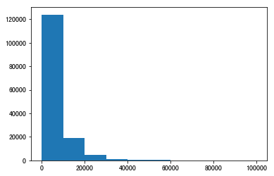
#### 3) 统计标签的基本分布信息
|
||
|
||
|
||
```python
|
||
print('Sta of label:')
|
||
Sta_inf(Y_data)
|
||
```
|
||
|
||
Sta of label:
|
||
_min 11
|
||
_max: 99999
|
||
_mean 5923.32733333
|
||
_ptp 99988
|
||
_std 7501.97346988
|
||
_var 56279605.9427
|
||
|
||
|
||
|
||
```python
|
||
## 绘制标签的统计图,查看标签分布
|
||
plt.hist(Y_data)
|
||
plt.show()
|
||
plt.close()
|
||
```
|
||
|
||
|
||

|
||
|
||
|
||
#### 4) 缺省值用-1填补
|
||
|
||
|
||
```python
|
||
X_data = X_data.fillna(-1)
|
||
X_test = X_test.fillna(-1)
|
||
```
|
||
|
||
### Step 4:模型训练与预测
|
||
|
||
#### 1) 利用xgb进行五折交叉验证查看模型的参数效果
|
||
|
||
|
||
```python
|
||
## xgb-Model
|
||
xgr = xgb.XGBRegressor(n_estimators=120, learning_rate=0.1, gamma=0, subsample=0.8,\
|
||
colsample_bytree=0.9, max_depth=7) #,objective ='reg:squarederror'
|
||
|
||
scores_train = []
|
||
scores = []
|
||
|
||
## 5折交叉验证方式
|
||
sk=StratifiedKFold(n_splits=5,shuffle=True,random_state=0)
|
||
for train_ind,val_ind in sk.split(X_data,Y_data):
|
||
|
||
train_x=X_data.iloc[train_ind].values
|
||
train_y=Y_data.iloc[train_ind]
|
||
val_x=X_data.iloc[val_ind].values
|
||
val_y=Y_data.iloc[val_ind]
|
||
|
||
xgr.fit(train_x,train_y)
|
||
pred_train_xgb=xgr.predict(train_x)
|
||
pred_xgb=xgr.predict(val_x)
|
||
|
||
score_train = mean_absolute_error(train_y,pred_train_xgb)
|
||
scores_train.append(score_train)
|
||
score = mean_absolute_error(val_y,pred_xgb)
|
||
scores.append(score)
|
||
|
||
print('Train mae:',np.mean(score_train))
|
||
print('Val mae',np.mean(scores))
|
||
```
|
||
|
||
Train mae: 628.086664863
|
||
Val mae 715.990013454
|
||
|
||
|
||
#### 2) 定义xgb和lgb模型函数
|
||
|
||
|
||
```python
|
||
def build_model_xgb(x_train,y_train):
|
||
model = xgb.XGBRegressor(n_estimators=150, learning_rate=0.1, gamma=0, subsample=0.8,\
|
||
colsample_bytree=0.9, max_depth=7) #, objective ='reg:squarederror'
|
||
model.fit(x_train, y_train)
|
||
return model
|
||
|
||
def build_model_lgb(x_train,y_train):
|
||
estimator = lgb.LGBMRegressor(num_leaves=127,n_estimators = 150)
|
||
param_grid = {
|
||
'learning_rate': [0.01, 0.05, 0.1, 0.2],
|
||
}
|
||
gbm = GridSearchCV(estimator, param_grid)
|
||
gbm.fit(x_train, y_train)
|
||
return gbm
|
||
```
|
||
|
||
#### 3)切分数据集(Train,Val)进行模型训练,评价和预测
|
||
|
||
|
||
```python
|
||
## Split data with val
|
||
x_train,x_val,y_train,y_val = train_test_split(X_data,Y_data,test_size=0.3)
|
||
```
|
||
|
||
|
||
```python
|
||
print('Train lgb...')
|
||
model_lgb = build_model_lgb(x_train,y_train)
|
||
val_lgb = model_lgb.predict(x_val)
|
||
MAE_lgb = mean_absolute_error(y_val,val_lgb)
|
||
print('MAE of val with lgb:',MAE_lgb)
|
||
|
||
print('Predict lgb...')
|
||
model_lgb_pre = build_model_lgb(X_data,Y_data)
|
||
subA_lgb = model_lgb_pre.predict(X_test)
|
||
print('Sta of Predict lgb:')
|
||
Sta_inf(subA_lgb)
|
||
```
|
||
|
||
Train lgb...
|
||
MAE of val with lgb: 689.084070621
|
||
Predict lgb...
|
||
Sta of Predict lgb:
|
||
_min -519.150259864
|
||
_max: 88575.1087721
|
||
_mean 5922.98242599
|
||
_ptp 89094.259032
|
||
_std 7377.29714126
|
||
_var 54424513.1104
|
||
|
||
|
||
|
||
```python
|
||
print('Train xgb...')
|
||
model_xgb = build_model_xgb(x_train,y_train)
|
||
val_xgb = model_xgb.predict(x_val)
|
||
MAE_xgb = mean_absolute_error(y_val,val_xgb)
|
||
print('MAE of val with xgb:',MAE_xgb)
|
||
|
||
print('Predict xgb...')
|
||
model_xgb_pre = build_model_xgb(X_data,Y_data)
|
||
subA_xgb = model_xgb_pre.predict(X_test)
|
||
print('Sta of Predict xgb:')
|
||
Sta_inf(subA_xgb)
|
||
```
|
||
|
||
Train xgb...
|
||
MAE of val with xgb: 715.37757816
|
||
Predict xgb...
|
||
Sta of Predict xgb:
|
||
_min -165.479
|
||
_max: 90051.8
|
||
_mean 5922.9
|
||
_ptp 90217.3
|
||
_std 7361.13
|
||
_var 5.41862e+07
|
||
|
||
|
||
#### 4)进行两模型的结果加权融合
|
||
|
||
|
||
```python
|
||
## 这里我们采取了简单的加权融合的方式
|
||
val_Weighted = (1-MAE_lgb/(MAE_xgb+MAE_lgb))*val_lgb+(1-MAE_xgb/(MAE_xgb+MAE_lgb))*val_xgb
|
||
val_Weighted[val_Weighted<0]=10 # 由于我们发现预测的最小值有负数,而真实情况下,price为负是不存在的,由此我们进行对应的后修正
|
||
print('MAE of val with Weighted ensemble:',mean_absolute_error(y_val,val_Weighted))
|
||
```
|
||
|
||
MAE of val with Weighted ensemble: 687.275745703
|
||
|
||
|
||
|
||
```python
|
||
sub_Weighted = (1-MAE_lgb/(MAE_xgb+MAE_lgb))*subA_lgb+(1-MAE_xgb/(MAE_xgb+MAE_lgb))*subA_xgb
|
||
|
||
## 查看预测值的统计进行
|
||
plt.hist(Y_data)
|
||
plt.show()
|
||
plt.close()
|
||
```
|
||
|
||
|
||
|
||
|
||
|
||
#### 5)输出结果
|
||
|
||
|
||
```python
|
||
sub = pd.DataFrame()
|
||
sub['SaleID'] = X_test.SaleID
|
||
sub['price'] = sub_Weighted
|
||
sub.to_csv('./sub_Weighted.csv',index=False)
|
||
```
|
||
|
||
|
||
```python
|
||
sub.head()
|
||
```
|
||
|
||
|
||
|
||
|
||
<div>
|
||
<style scoped>
|
||
.dataframe tbody tr th:only-of-type {
|
||
vertical-align: middle;
|
||
}
|
||
|
||
.dataframe tbody tr th {
|
||
vertical-align: top;
|
||
}
|
||
|
||
.dataframe thead th {
|
||
text-align: right;
|
||
}
|
||
</style>
|
||
<table border="1" class="dataframe">
|
||
<thead>
|
||
<tr style="text-align: right;">
|
||
<th></th>
|
||
<th>SaleID</th>
|
||
<th>price</th>
|
||
</tr>
|
||
</thead>
|
||
<tbody>
|
||
<tr>
|
||
<th>0</th>
|
||
<td>0</td>
|
||
<td>39533.727414</td>
|
||
</tr>
|
||
<tr>
|
||
<th>1</th>
|
||
<td>1</td>
|
||
<td>386.081960</td>
|
||
</tr>
|
||
<tr>
|
||
<th>2</th>
|
||
<td>2</td>
|
||
<td>7791.974571</td>
|
||
</tr>
|
||
<tr>
|
||
<th>3</th>
|
||
<td>3</td>
|
||
<td>11835.211966</td>
|
||
</tr>
|
||
<tr>
|
||
<th>4</th>
|
||
<td>4</td>
|
||
<td>585.420407</td>
|
||
</tr>
|
||
</tbody>
|
||
</table>
|
||
</div>
|
||
|
||
|
||
|
||
**Baseline END.**
|
||
|
||
--- By: ML67
|
||
|
||
Email: maolinw67@163.com
|
||
PS: 华中科技大学研究生, 长期混迹Tianchi等,希望和大家多多交流。
|
||
github: https://github.com/mlw67 (近期会做一些书籍推导和代码的整理)
|
||
|
||
--- By: AI蜗牛车
|
||
|
||
PS:东南大学研究生,研究方向主要是时空序列预测和时间序列数据挖掘
|
||
公众号: AI蜗牛车
|
||
知乎: https://www.zhihu.com/people/seu-aigua-niu-che
|
||
github: https://github.com/chehongshu
|
||
|
||
--- By: 阿泽
|
||
|
||
PS:复旦大学计算机研究生
|
||
知乎:阿泽 https://www.zhihu.com/people/is-aze(主要面向初学者的知识整理)
|
||
|
||
--- By: 小雨姑娘
|
||
|
||
PS:数据挖掘爱好者,多次获得比赛TOP名次。
|
||
知乎:小雨姑娘的机器学习笔记:https://zhuanlan.zhihu.com/mlbasic
|
||
|
||
**关于Datawhale:**
|
||
|
||
> Datawhale是一个专注于数据科学与AI领域的开源组织,汇集了众多领域院校和知名企业的优秀学习者,聚合了一群有开源精神和探索精神的团队成员。Datawhale 以“for the learner,和学习者一起成长”为愿景,鼓励真实地展现自我、开放包容、互信互助、敢于试错和勇于担当。同时 Datawhale 用开源的理念去探索开源内容、开源学习和开源方案,赋能人才培养,助力人才成长,建立起人与人,人与知识,人与企业和人与未来的联结。
|
||
|
||
本次数据挖掘路径学习,专题知识将在天池分享,详情可关注Datawhale:
|
||
|
||

|
||
|
||
|